Belief-Conditioned One-Step Diffusion: Real-Time Trajectory Planning with Just-Enough Sensing
1 University of Illinois Urbana-Champaign (UIUC)
2 University of Florida (UF)
3 Florida International University (FIU)
Accepted to CoRL as an Oral paper (top 5%)
Corresponding author: Gokul Puthumanaillam
Abstract
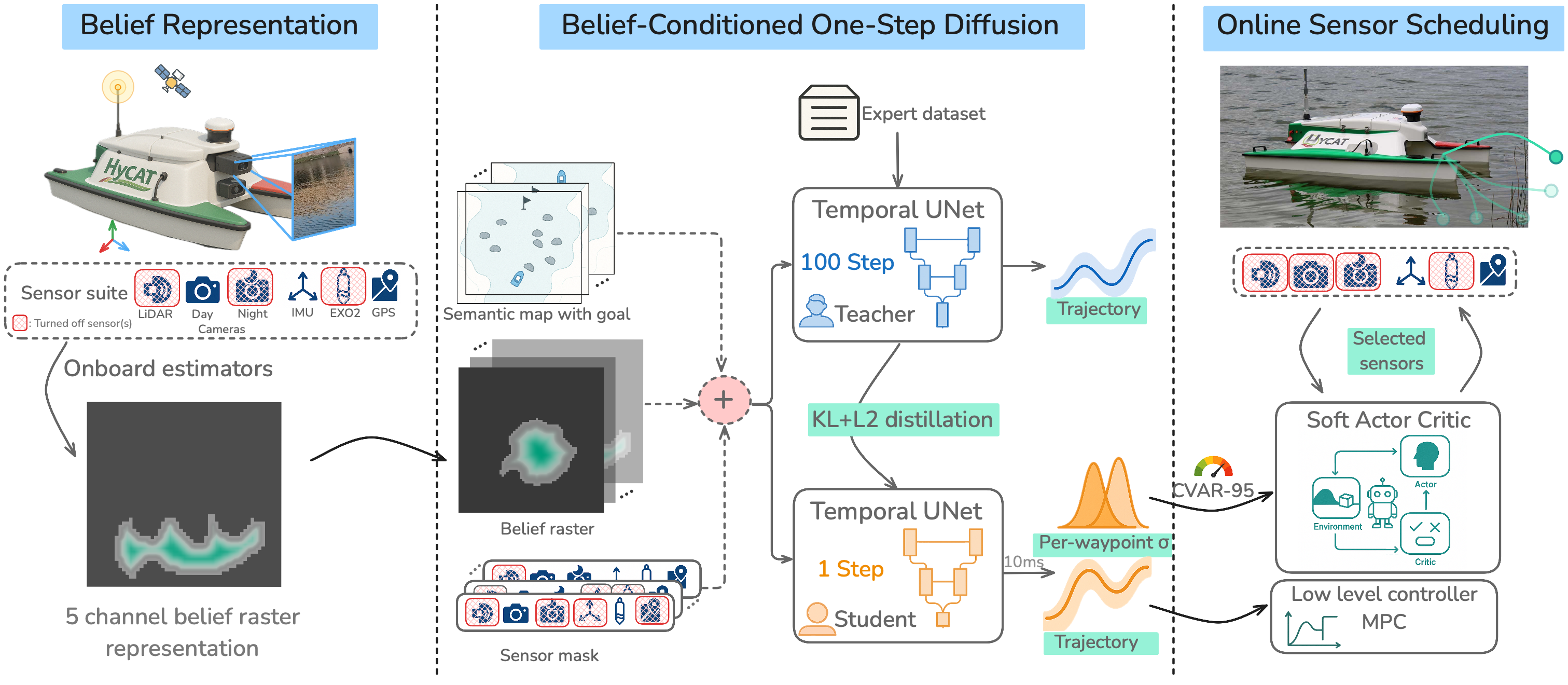
Robots equipped with rich sensor suites can localize reliably in partially-observable environments---but powering every sensor continuously is wasteful and often infeasible. Belief-space planners address this by propagating pose-belief covariance through analytic models and switching sensors heuristically--a brittle, runtime-expensive approach. Data-driven approaches--including diffusion models--learn multi-modal trajectories from demonstrations, but presuppose an accurate, always-on state estimate. We address the largely open problem: for a given task in a mapped environment, which minimal sensor subset must be active at each location to maintain state uncertainty just low enough to complete the task? Our key insight is that when a diffusion planner is explicitly conditioned on a pose-belief raster and a sensor mask, the spread of its denoising trajectories yields a calibrated, differentiable proxy for the expected localisation error. Building on this insight, we present Belief-Conditioned One-Step Diffusion (B-COD), the first planner that, in a 10 ms forward pass, returns a short-horizon trajectory, per-waypoint aleatoric variances, and a proxy for localisation error--eliminating external covariance rollouts. We show that this single proxy suffices for a soft-actor-critic to choose sensors online, optimising energy while bounding pose-covariance growth. We deploy B-COD in real-time marine trials on an unmanned surface vehicle and show that it reduces sensing energy consumption while matching the goal-reach performance of an always-on baseline.
Methodology
Real-World Experiments (Qualitative Results)
Our evaluation targets a real-world, real-time scenario in which an autonomous surface vehicle (ASV) must navigate a previously unseen open-air lake to reach waypoint goals with just-enough sensing while keeping the CVaR-95 localisation error below a user budget of 2 m. The lake presents both natural and human-driven disturbances: winds, waves, fountains, floating buoys and human-induced sensor denied zones. The test platform is a SeaRobotics Surveyor ASV with a differential-thrust propulsion module and a heterogeneous sensor suite: a multi-beam LiDAR, day and night cameras, RTK-GPS, MEMS IMU, and an EXO2 sonde. Control inputs are augmented by a discrete mode flag that selects the estimator configuration implied by the powered sensors. Sensor power draw differs by an order of magnitude, so efficient scheduling has tangible impact on total mission energy.
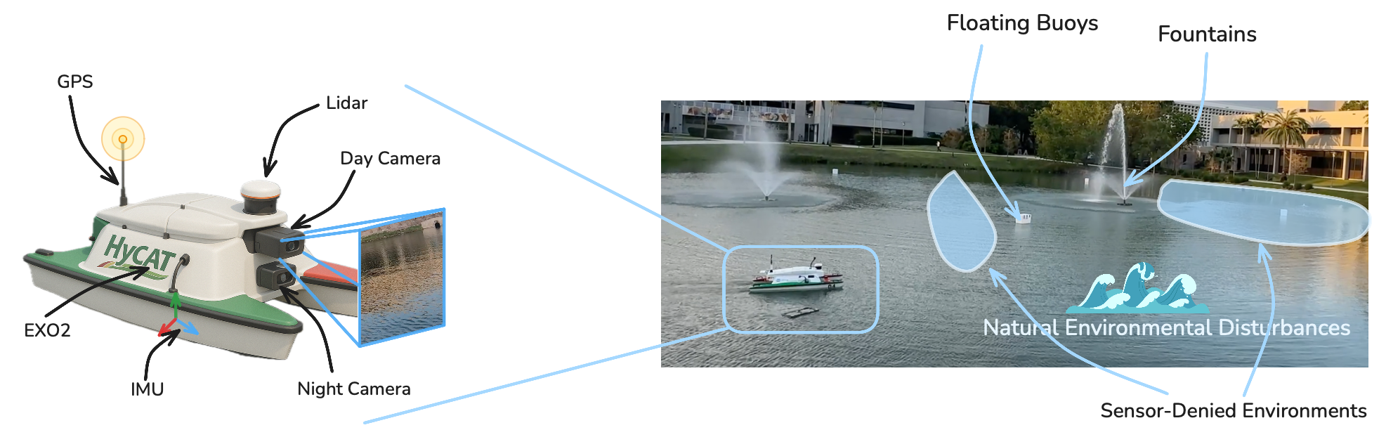
Environment and Autonomous Surface Vehicle testbed
Experiment videos
Click on the videos below to view the experiments (the videos are sped up for brevity).
Experiment 1 (Day Lap): ASV navigating in an environment with a human induced sensor (GPS) denied zone and a EXO2 rich zone.
Experiment 2 (Night Lap): ASV navigating in the environment during night time.
Experiment 3 (Night Lap): ASV navigating in the environment during night time.
Experiment 4 (Day Lap): ASV navigating in the environment but we force LiDAR to be off in an obstacle rich zone (where LiDAR is usually heavily used).
Key Findings (Quantitative Results)
Click on the images below to view the detailed key findings.
| Metric | Always-ON | B-COD+SAC |
|---|---|---|
| Goal-reach (%) | 100.0 | 97.9 |
| Collision (%) | 0.5 | 0.9 |
| CVaR violations (%) | 0.1 | 0.5 |
| Mean #sensors | 5.0 | 2.08 |
| Energy vs AON (%) | 100.0 | 42.3 |
| Runtime (ms) | 14.9 | 14.3 |
| Peak RAM (MB) | 305 | 284 |
| r (m) | B-COD | IGG | DL |
|---|---|---|---|
| 25 | 9.8 ms | 7.5 ms | 565 ms |
| 40 | 9.7 ms | 10.9 ms | 1446 ms |
| 55 | 9.6 ms | 14.6 ms | 2737 ms |
| 70 | 10.7 ms | 18.2 ms | 4430 ms |
| 85 | 10.4 ms | 18.7 ms | 6536 ms |
| 100 | 10.9 ms | 23.3 ms | 9040 ms |
Key Finding #1: B-COD+SAC delivers near-perfect task completion at less than half the sensing cost of the Always-ON baseline.
| Metric | AON | GOF | IGG | R1 | R2 | σM | SS | NB | PRL | DL | Ours |
|---|---|---|---|---|---|---|---|---|---|---|---|
| Goal-reach (%) | 100.0 | 47.3 | 89.9 | 18.5 | 29.1 | 79.6 | 94.3 | 67.8 | 54.8 | 87.9 | 97.9 |
| Collision (%) | 0.5 | 22.3 | 6.1 | 34.5 | 30.1 | 12.4 | 4.7 | 17.4 | 22.1 | 4.2 | 0.9 |
| CVaR violations (%) | 0.1 | 15.8 | 4.3 | 28.6 | 22.8 | 9.1 | 5.2 | 13.2 | 18.3 | 1.9 | 0.5 |
| Mean #sensors | 5.0 | 3.19 | 2.65 | 1.0 | 2.0 | 2.99 | 2.56 | 4.05 | 3.48 | 5.0 | 2.08 |
| Energy vs AON (%) | 100.0 | 61.2 | 49.8 | 24.2 | 38.9 | 60.1 | 91.2 | 68.2 | 67.5 | 100 | 42.3 |
| Runtime (ms) | 14.9 | 14.7 | 26.8 | 13.6 | 13.7 | 14.4 | 84.1 | 14.1 | 12.1 | 565.3 | 14.3 |
| Peak RAM (MB) | 305 | 282 | 403 | 277 | 281 | 287 | 674 | 279 | 299 | 731 | 284 |
Table above summarizes performance over 50 laps. B-COD reaches the goal on 97.9 \% of attempts, yet spends only 42% of the energy. Collisions remain at 0.9%, essentially identical to the Always-ON baseline. Heuristic scheduling cannot match this trade-off: Greedy-OFF conserves energy (61%) but sacrifices success (47%). InfoGain-Greedy raises success to 90% yet violates risk eight times more often than B-COD. Random masks fare worse, proving that local environment context--not just a lower duty cycle--is essential for task completion. Pure-RL generates trajectories and schedules sensors from raw rasters; the high-dimensional action space makes exploration sparse, and the policy converges to risk-averse dithering--only 55% goals reached and a 22% collision rate. DESPOT-Lite, by contrast, evaluates a principled belief tree with analytic models and therefore is able to plan accurately, but it expands hundreds of nodes; the resulting 0.5s runtime renders it unusable in real-time on the vehicle.
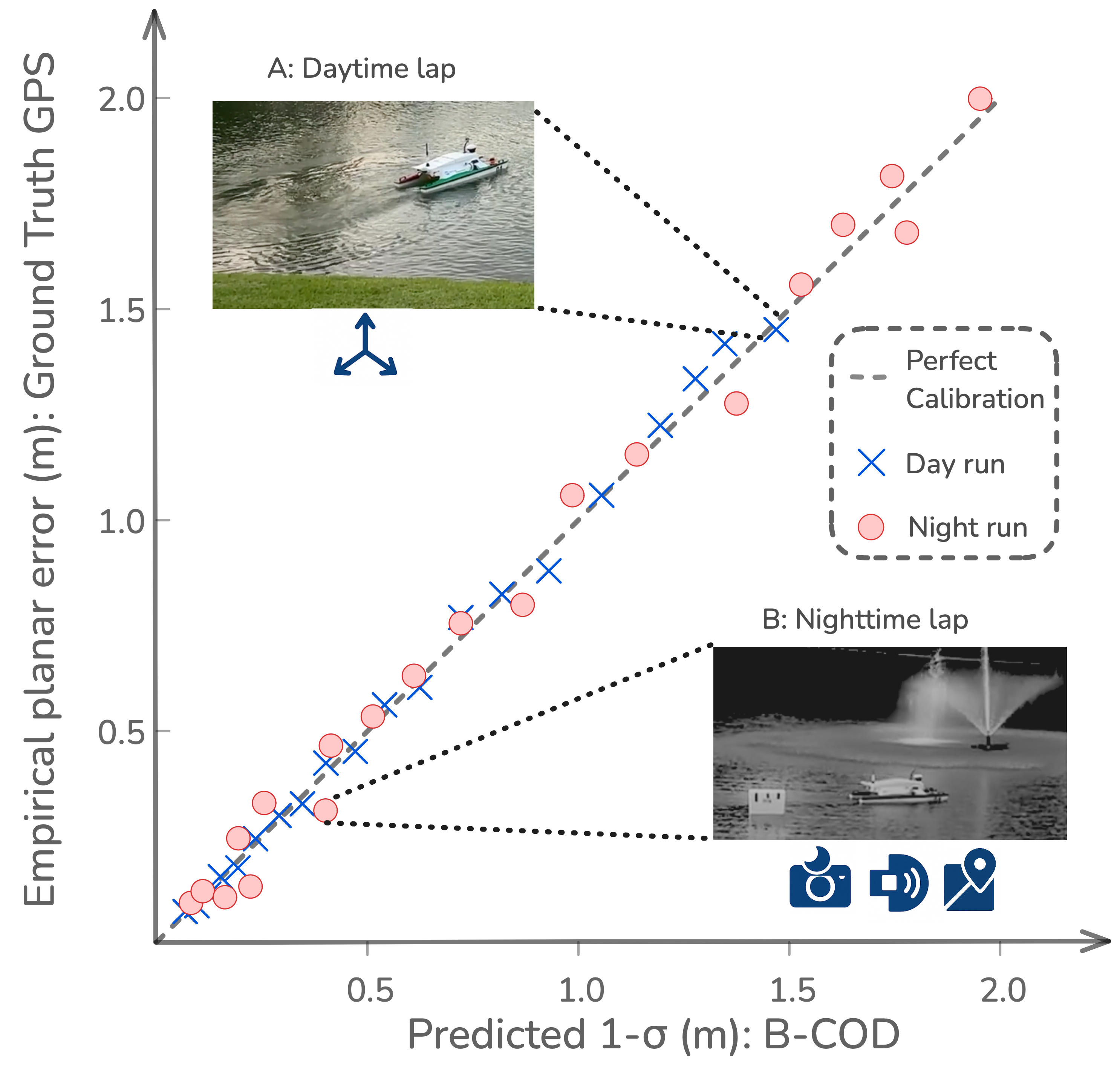
Key Finding #2: B-COD's variance is a calibrated, context-aware predictor of localisation error.
The reliability curve shows numerical calibration (6 mean error). The reason behind the bound relaxing follows directly from what the diffusion planner is told to care about: belief shape, active sensors, and local map geometry. Call-out B (night lap, obstacle corridor): The semantic map reports obstacles--a fountain and a floating buoy. Colliding here would be mission-ending, so B-COD turns on LiDAR, night camera and IMU (high energy). The planner now expects rich pose updates and knows that centimeters of pose error matter; it shrinks the bound to 0.45 m, almost matching the 0.46 m ground truth drift. Call-out A (day lap): Tens of meters separate the ASV from any hazard. With only the IMU running (low energy), B-COD predicts pure dead-reckoning growth yet also "knows" that a meter of drift will not intersect anything. It therefore widens the bound to 1.85 m, closely tracking the ground truth 2.0 m error. These results demonstrate that u^CVaR is numerically reliable and spatially discriminative, providing the scheduler with the rich information needed to trade energy for certainty.
Key Finding #3: B-COD stays within a 10 ± 1 ms envelope and out-scales analytic belief planners.
| r (m) | B-COD | IGG | DL |
|---|---|---|---|
| 25 | 9.8 ms | 7.5 ms | 565 ms |
| 40 | 9.7 ms | 10.9 ms | 1446 ms |
| 55 | 9.6 ms | 14.6 ms | 2737 ms |
| 70 | 10.7 ms | 18.2 ms | 4430 ms |
| 85 | 10.4 ms | 18.7 ms | 6536 ms |
| 100 | 10.9 ms | 23.3 ms | 9040 ms |
The table above sweeps the workspace radius from 25 m to 100 m (full lake sector). B-COD's latency is flat--10.3 +- 0.6 ms throughout—because the belief crop is always down-sampled and the UNet's receptive field is fixed; compute therefore scales with network width, not with world area. The InfoGain-Greedy baseline must update an n-cell covariance grid; its cost grows \Theta(R^{2}), reaching 23 ms at 100 m. DESPOT-Lite's branching factor of the belief tree increases with visible free space; runtime balloons to 9000 ms over the same sweep, far beyond what an embedded loop can absorb. The takeaway is practical as well as theoretical: constant-time scaling lets B-COD replan over lake-scale horizons without ever violating the real-time threshold, whereas analytic planners become the computational bottleneck well before the map reaches lake-scale.
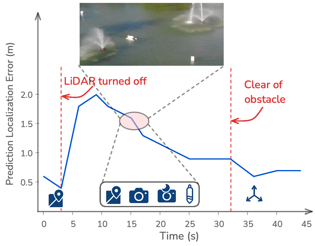
Key Finding #4: B-COD adapts online, re-allocating modalities to recover from faults.
During a daytime lap, we manually disabled the LiDAR 30 seconds before the ASV entered the narrow fountain corridor, which demands typically sub-meter localisation. B-COD's risk proxy spiked from 0.6 m to 1.8 m as soon as the loss of range data was reflected. The SA reacted on the next cycle: it re-enabled both cameras and the EXO2 sonde, accepted the high energy penalty, and drove risk down to 0.8 m. Once clear of the obstacle, the proxy dropped naturally; the scheduler shut the extra modalities off and returned to the energy-saving IMU-only sensor choice. No heuristic or fault-flag was required--the planner's calibrated variance alone drove the correct, context-specific recovery sequence.
Dataset
Our dataset consists of field logs collected from freshwater lake operations, including twelve day-time and eight night-time sorties. The SeaRobotics Surveyor ASV collected:
- 32-beam spinning LiDAR point clouds (10 Hz, ROS/PCD)
- RGB images (20 Hz, PNG)
- Near-IR images under 850 nm active illumination (20 Hz, PNG)
- RTK-GNSS fixes (5 Hz, NMEA)
- Six-axis IMU messages (200 Hz, ROS/Imu)
- Water-quality probe samples (2 Hz, CSV)
All topics share a chronologically consistent ROS /clock, with each log accompanied by recordings of wind and irradiance for domain-randomisation replay.
An annonymous subset of the dataset (15GB) is available for download (anonymization takes time and hence we chose to release a subset and not the whole dataset): https://github.com/bcod-diffusion/dataset. We plan to release the whole dataset (280GB) under a Creative Commons Attribution-NonCommercial-ShareAlike 4.0 International License (CC BY-NC-SA 4.0).
Real→Sim Transfer
Logs are imported into an in-house Unity 2022.3 + ROS 2 simulator that reconstructs the shoreline mesh, static obstacles, bathymetry and approximate above-surface lighting. Dynamic objects are re-instantiated with ground-truth trajectories.
Dataset Statistics
- Modalities: 100% contain LiDAR and IMU; day camera appears in 72%, night camera in 28%, GNSS in 64%, sonde in 18%
- Belief spread: Median planar 1σ = 0.38 m; 95th percentile = 2.1 m
- Lighting: Illumination spans 0.2–55 kLux; clips are evenly stratified into five bins for training/validation
- Obstacles: Each snippet is annotated with the minimum range to shoreline and to floating hazards; mean 14.2 m, min 0.8 m
EXO2 and GPS Data Visualization
LiDAR Point Cloud Visualization
Camera Feed Visualization
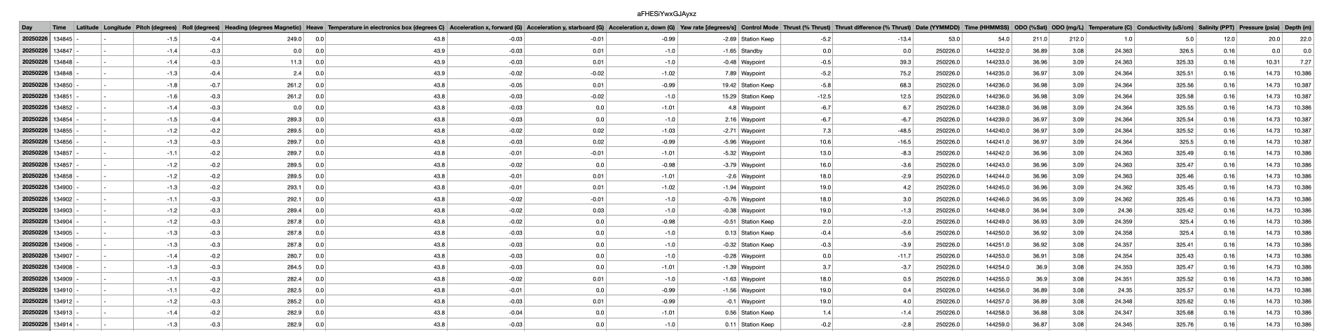
EXO2 and GPS Data
Example CSV file of EXO2 water quality probe data and GPS measurements collected during lake operations.
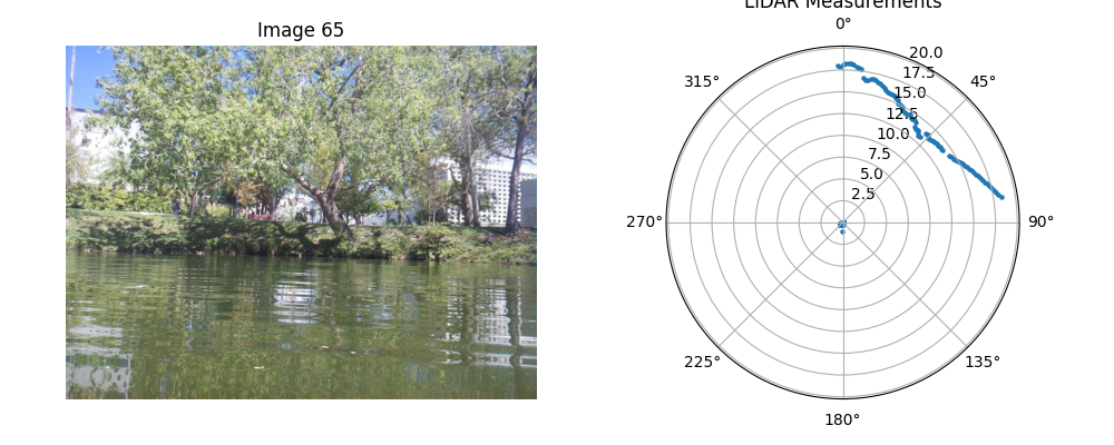
LiDAR Point Cloud
LiDAR point cloud data collected at 10 Hz, providing environmental mapping.
Camera Feed
RGB camera (night camera in this case) feed showing real-time environmental perception.
Built with ❤ by the B-COD Team
For questions and collaborations, contact: gokulp2@illinois.edu
BibTeX
@inproceedings{Puthumanaillam2025BCoD,
  title     = {Belief-Conditioned One-Step Diffusion: Real-Time Trajectory Planning with Just-Enough Sensing},
  author    = {Gokul Puthumanaillam and Aditya Penumarti and Manav Vora and Paulo Padrao and Jose Fuentes and Leonardo Bobadilla and Jane Shin and Melkior Ornik},
  booktitle = {Conference on Robot Learning (CoRL)},
  year      = {2025},
  note      = {Oral (top 5%)},
  url       = {https://github.com/bcod-diffusion/bcod-diffusion.github.io/blob/main/paper.pdf}
}